Result Analysis
Contents
VMD
Free space visual inspection
The first thing to do when Epock calculation is done is probably to check
that the free space detected fits well the pocket.
This can be easily done using Epock option to output the free space as a
topology and a trajectory file (--ox option).
The protein and the free space trajectories can be loaded at the same time
in VMD:
$ vmd prot.pdb prot.xtc -f cav.pdb cav.xtc
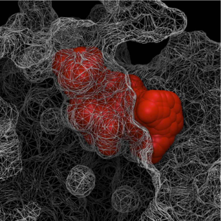
A rapid visual inspection can be easily done representing the protein as a
wireframe surface and the free space as van der Walls spheres.
Note that, a more accurate visual inspection can be done by making sure VMD
uses the same van der Walls radii as Epock.
For the free space, Epock uses a van der Walls radius of 1.4 Å
(parameter padding in Epock configuration files).
To do so, open the VMD Tk console (Extensions -> Tk Console) and type
% [atomselect 1 "all"] set radius 1.4
On the figure below, we can see that Epock perfectly detected the free space volume that lies between the protein atoms. In that sense, Epock reproduces VMD’ results.
When running Epock from VMD, after pushing the “calculate volume” button on the tab “static analysis” and the calculation is done, a new window appears.
The “static” result window
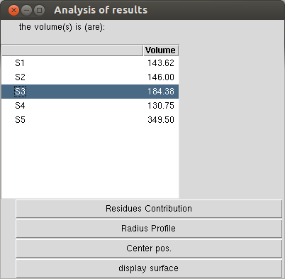
Result window that open after a static volume calculation. The volume value calculated for each pocket appears in the table.
More results can be display hitting the bottom buttons:
“Residues contribution” opens a new window with the list residues involved in the pocket (see also residue contribution analysis).
“Radius profile” gives the radius profile of the pore (see also profile analysis).
“Center pos” loads the pdb file of the calculated center of the pore (for a pore profile analysis again),
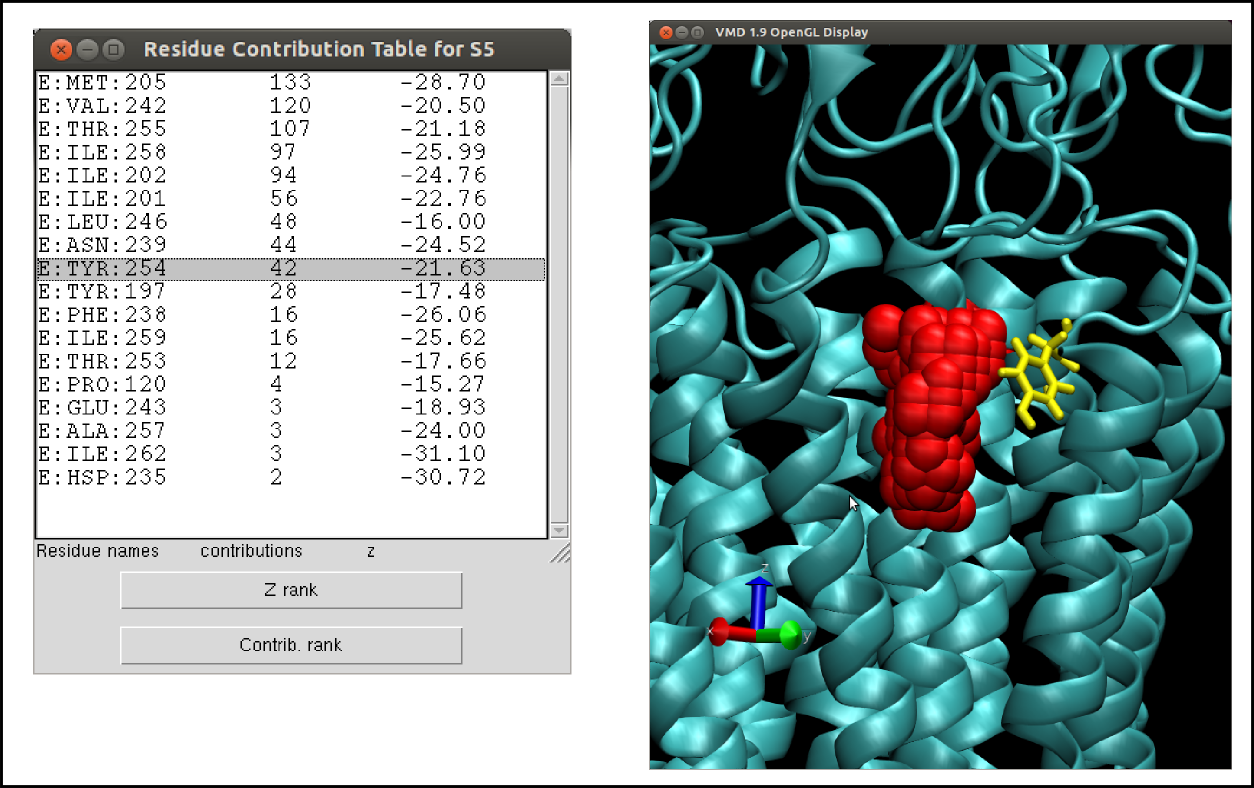
Residue contribution window (left) and OpenGL window (right). Clicking a residue in the list displays it in yellow sticks in the OpenGL window.
The “dynamic” result window
The dynamic analysis results work pretty much the same as static analysis.

Result window that open after a dynamic volume calculation (i.e. a volume calculation along a trajectory). It looks actually very similar than for a single frame analysis!
“Volume vs Time” quite explicit isn’t it?
“Residue contribution” will, in addition to what it does for a static analysis, allow the user to plot the contribution of a specific residue versus time.
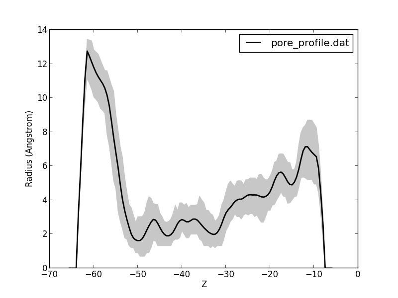
“Radius profile” plots the average radius as well as the min and max for each z value (valuable for a pore).
“Center pos” will do the same as for a static analysis i.e. add red spheres located in the calculated center of the pore.
Python Scripts
Please note that these Python scripts require:
- Python version 2.7.x, the Python interpreter
- matplotlib version >= 1.1.1, the Python plot library
- Numpy version >= 1.6.1, a package for scientific computing with Python
plot.py
Description
This script draws a timeline plot of each pocket volume in each file passed to command-line.
Usage
$ python plot.py -h
usage: plot.py [-h] [-o OUTPUT] filename [filename ...]

This script draws a timeline plot of each pocket volume in each file passed to
command-line.

positional arguments:
  filename                    volume data file

optional arguments:
  -h, --help                  show this help message and exit
  -o OUTPUT, --output OUTPUT  output file name
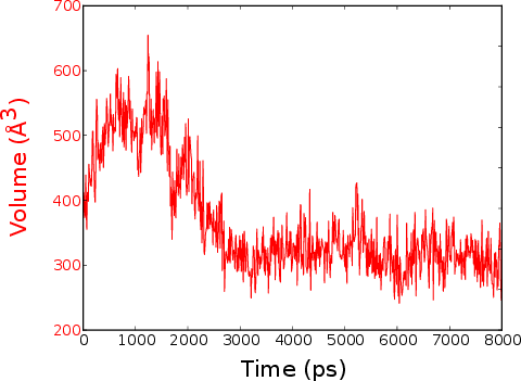
plot_contribution.py
Description
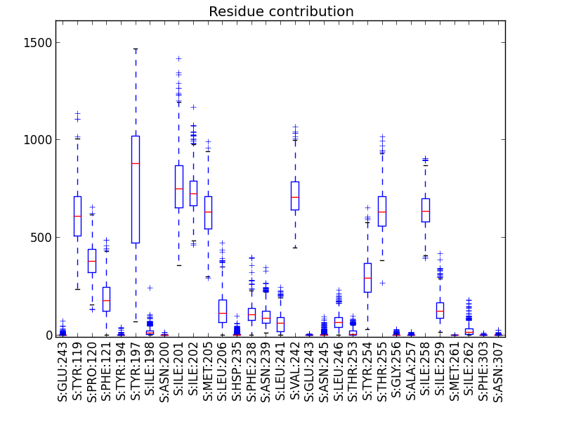
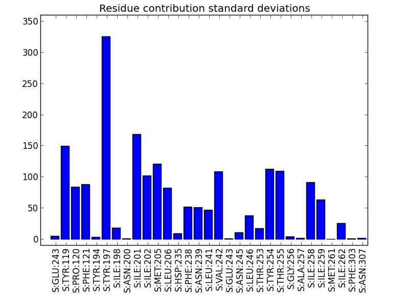
This script aims to visualize Epock’s residue contribution output file (see residue contribution analysis).
There are several complementary ways to use this plot these data:
- a box plot showing each residue contribution median and standard deviation (default),
- a bar plot showing only standard deviations (
-s, --stdevoption), - a timeline plot showing a specific residue contribution versus time (
-roption).
Usage
python plot_contribution.py -h
usage: plot_contribution.py [-h] [-o OUTPUT] [-n N] [-s]
                            [-r residue [residue ...]]
                            filename

This script draws a boxplot of each atom contribution to the cavity.

positional arguments:
  filename                    contribution data file

optional arguments:
  -h, --help                  show this help message and exit
  -o OUTPUT, --output OUTPUT  output file name
  -n N                        show n greatest contributions
  -s, --stdev                 only plot standard deviations
  -r residue [residue ...]    plot specific residues along time

plot_profile.py
Description
This script aims to visualize Epock’s residue contribution output file (see profile analysis).
This script plots the minimum, maximum and average profile from a profile file passed to command-line.
Usage
usage: plot_profile.py [-h] [-o OUTPUT] filename [filename ...]

This script plots the minimum, maximum and average profile from a profile file
passed to command-line.

positional arguments:
  filename                    contribution data file

optional arguments:
  -h, --help                  show this help message and exit
  -o OUTPUT, --output OUTPUT  output file name